Chapter 5 Plotting differential abundance data

A couple of plots to explore differential abundance data are generated using additional custom functions

5.1 Volcano plots

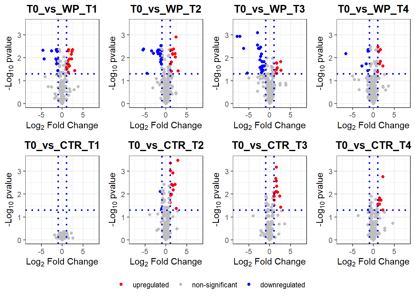
Volcano plots are used to visualize the up- and downregulated features identified during the differential abundance analysis. Volcanos will be obtained using the plot_volcano() custom function. Because there are multiple comparisons a for() loop will be used to generate multiple volcano plots that will be arranged together with ggarrange().

library(ggpubr)
plot_list <- list()

for(comp in unique(diff_table$comparison)){
  volcano_plot <- diff_table %>% 
  filter(comparison == comp) %>% 
  plot_volcano(.,
               column_with_log2FC = log2FC,
               column_with_pval = pval.adj,
               log2FC.threshold = 1,
               pval.threshold = 0.05) +
    scale_x_continuous(limits = c(-8, 8)) +
    scale_y_continuous(limits = c(0, 3.5)) +
    labs(title = comp)
  
  plot_list[[length(plot_list) + 1]] <- volcano_plot
}

ggarrange(plotlist = plot_list, ncol = 4, nrow = 2, common.legend = TRUE, legend = 'bottom')

## Warning: Removed 1 rows containing missing values (geom_point).

Figure 5.1: Volcano plots of metabolite data